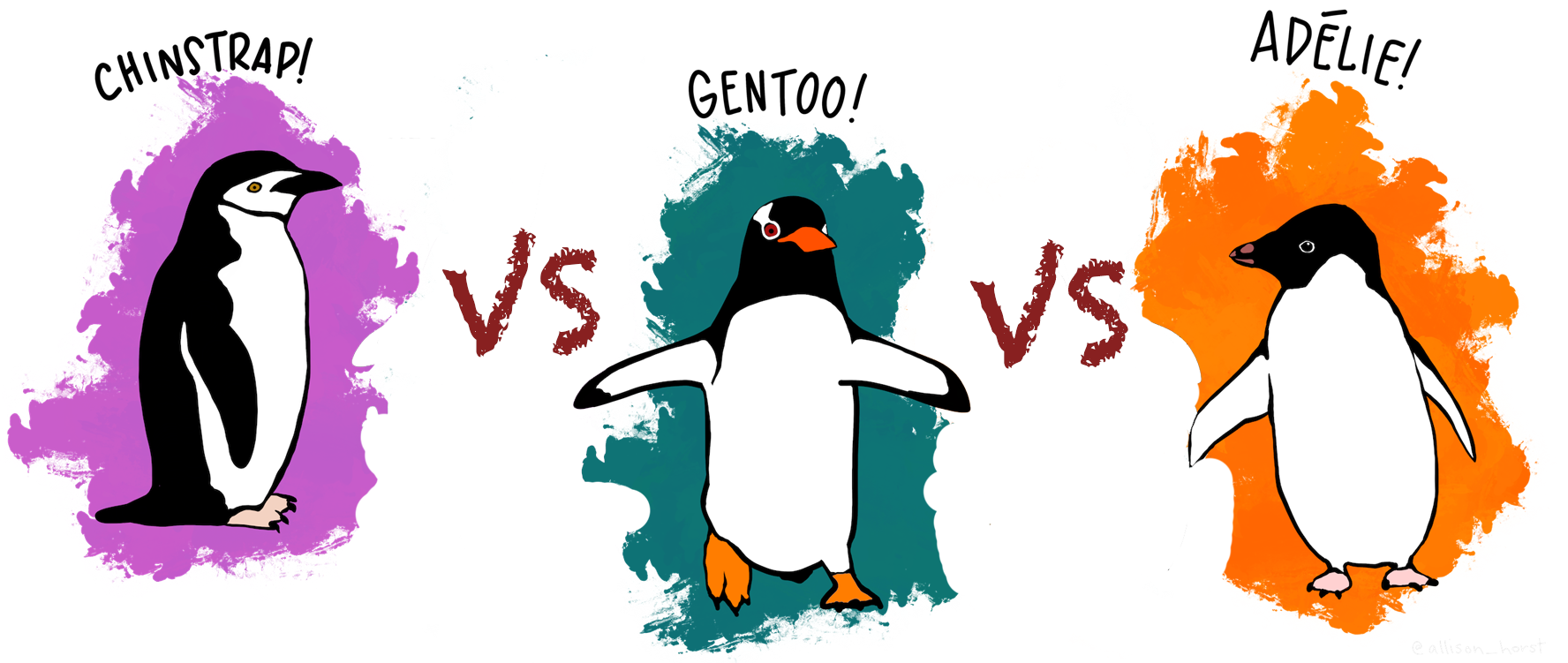
I will give a short overview of the most common ways to encode a categorical variables. To make the whole exercise more fun, I will will use the awesome palmerpenguins package by Allison Horst. Because who doesn’t like penguins :)
Preparation
# Load some helper packages
library(tidyverse, warn.conflicts = FALSE)
# Load data (install from https://github.com/allisonhorst/palmerpenguins)
library(palmerpenguins)
# Set global theme
theme_set(cowplot::theme_cowplot() +
            theme(axis.title.x = element_blank()))
The data contains data on 344 penguins from three different species. We will compare the size of their flippers:
# Filter out some missing values and take a subset
peng <- drop_na(penguins)[1:290, ] %>%
  arrange(species)

# example row numbers for individuals from each species
selection <- c(1:3, 147:150, 172:175)

ggplot(peng, aes(x=species, y = flipper_length_mm)) +
  ggbeeswarm::geom_beeswarm() +
  stat_summary(geom = "crossbar", color = "red", fun = mean, width = 0.2) +
  annotate("text", x = 2.85, hjust = 1, y = 217.5, label = "Group Mean", color = "red")
Dummy Coding
Dummy coding is the simplest way to encode a categorical variable. If we fit a linear model with the flipper length as response variable and use dummy coding for the species, each estimated coefficient will the mean length of that species:
model.matrix(~ species - 1, data = peng)[selection, ]## speciesAdelie speciesChinstrap speciesGentoo
## 1 1 0 0
## 2 1 0 0
## 3 1 0 0
## 147 0 1 0
## 148 0 1 0
## 149 0 1 0
## 150 0 1 0
## 172 0 0 1
## 173 0 0 1
## 174 0 0 1
## 175 0 0 1fit <- lm(flipper_length_mm ~ species - 1, data = peng)
coef(fit)## speciesAdelie speciesChinstrap speciesGentoo
## 190.1027 192.2400 217.2353ggplot(peng, aes(x=species, y = flipper_length_mm)) +
ggbeeswarm::geom_beeswarm() +
stat_summary(geom = "crossbar", color = "red", fun = mean, width = 0.2) +
geom_segment(data = data.frame(species = c("Adelie", "Chinstrap", "Gentoo"), coef = coef(fit)),
aes(xend = species, y = 170, yend = coef), color = "purple", size = 2) +
annotate("text", x = 2.95, y = 190, hjust = 1, label = "Coef_3", color = "purple") +
annotate("text", x = 1.95, y = 182, hjust = 1, label = "Coef_2", color = "purple") +
annotate("text", x = 0.95, y = 178, hjust = 1, label = "Coef_1", color = "purple") +
ggtitle("Dummy coding", subtitle = "Each parameter has is the mean of one group.\nNote that the model does not have an intercept.")
Treatment Contrast
Treatment contrast is the default in R for encoding a categorical variable if you include an intercept in the model:
model.matrix(~ species, data = peng, contrasts.arg = list(species = contr.treatment))[selection, ]## (Intercept) species2 species3
## 1 1 0 0
## 2 1 0 0
## 3 1 0 0
## 147 1 1 0
## 148 1 1 0
## 149 1 1 0
## 150 1 1 0
## 172 1 0 1
## 173 1 0 1
## 174 1 0 1
## 175 1 0 1fit2 <- lm(flipper_length_mm ~ species, data = peng, contrasts = list(species = contr.treatment))
coef(fit2)## (Intercept) species2 species3
## 190.10274 2.13726 27.13255ggplot(peng, aes(x=species, y = flipper_length_mm)) +
ggbeeswarm::geom_beeswarm() +
stat_summary(geom = "crossbar", color = "red", fun = mean, width = 0.2) +
geom_hline(yintercept = coef(fit2)[1], color = "purple") +
geom_segment(x="Chinstrap", xend = "Chinstrap", y = coef(fit2)[1], yend = coef(fit2)[1] + coef(fit2)[2],
color = "purple", size = 2) +
geom_segment(x="Gentoo", xend = "Gentoo", y = coef(fit2)[1], yend = coef(fit2)[1] + coef(fit2)[3],
color = "purple", size = 2) +
annotate("text", x = 0.8, y = 191, label = "Intercept", hjust = 1, vjust = 0, size = 4, color = "purple") +
annotate("text", x = 2.95, y = 200, hjust = 1, label = "Coef_3", color = "purple") +
ggtitle("Treatment Contrast", subtitle = "All groups are compared against a baseline level (the first level in a\nfactor which is often just the one starting with 'A').")
Sum Contrast
The sum contrast is useful if the intercept should encompass information from all groups. However, be careful the intercept is not necessarily equal to the mean over all observations. Instead it is the mean of the group-wise means.
model.matrix(~ species, data = peng, contrasts.arg = list(species = contr.sum))[selection, ]## (Intercept) species1 species2
## 1 1 1 0
## 2 1 1 0
## 3 1 1 0
## 147 1 0 1
## 148 1 0 1
## 149 1 0 1
## 150 1 0 1
## 172 1 -1 -1
## 173 1 -1 -1
## 174 1 -1 -1
## 175 1 -1 -1fit3 <- lm(flipper_length_mm ~ species, data = peng, contrasts = list(species = contr.sum))
coef(fit3)## (Intercept) species1 species2
## 199.859345 -9.756605 -7.619345ggplot(peng, aes(x=species, y = flipper_length_mm)) +
ggbeeswarm::geom_beeswarm() +
stat_summary(geom = "crossbar", color = "red", fun = mean, width = 0.2) +
geom_hline(yintercept = mean(peng$flipper_length_mm), color = "#cc0a1a") +
geom_hline(yintercept = coef(fit3)[1], color = "purple") +
geom_segment(x="Adelie", xend = "Adelie", y = coef(fit3)[1], yend = coef(fit3)[1] + coef(fit3)[2],
color = "purple", size = 2) +
geom_segment(x="Chinstrap", xend = "Chinstrap", y = coef(fit3)[1], yend = coef(fit3)[1] + coef(fit3)[3],
color = "purple", size = 2) +
annotate("text", x = 0.85, y = 203, label = "Overall\nMean", hjust = 1, vjust = 0, size = 4, color = "#cc0a1a", lineheight = 0.8) +
annotate("text", x = 0.85, y = 199, label = "Intercept", hjust = 1, vjust = 1, size = 4, color = "purple") +
annotate("text", x = 1.95, y = 196, hjust = 1, label = "Coef_3", color = "purple") +
ggtitle("Sum Contrast", subtitle = "The intercept is the mean of the group-means, the coefficients\nare the deviation from the mean.")
To calculate the third group mean, subtract both coefficients from the intercept:
mean(peng[peng$species == "Gentoo", ]$flipper_length_mm)
coef(fit3)[1] - coef(fit3)[2] - coef(fit3)[3]
## [1] 217.2353
## (Intercept)
## 217.2353Helmert Coding
Helmert coding is not really useful for categorical variables; it is however the default for ordered factors, which is why I decided to include it here. For ordered factors we don’t want to assume that each step is equidistant, so each coefficient encodes the difference to the average of the previous groups:
model.matrix(~ species, data = peng, contrasts.arg = list(species = contr.helmert))[selection, ]## (Intercept) species1 species2
## 1 1 -1 -1
## 2 1 -1 -1
## 3 1 -1 -1
## 147 1 1 -1
## 148 1 1 -1
## 149 1 1 -1
## 150 1 1 -1
## 172 1 0 2
## 173 1 0 2
## 174 1 0 2
## 175 1 0 2fit4 <- lm(flipper_length_mm ~ species, data = peng, contrasts = list(species = contr.helmert))
coef(fit4)## (Intercept) species1 species2
## 199.859345 1.068630 8.687975ggplot(peng, aes(x=species, y = flipper_length_mm)) +
ggbeeswarm::geom_beeswarm() +
stat_summary(geom = "crossbar", color = "red", fun = mean, width = 0.2) +
geom_hline(yintercept = mean(peng$flipper_length_mm), color = "#cc0a1a") +
geom_hline(yintercept = coef(fit3)[1], color = "purple") +
geom_segment(x = 0.7, xend = 2.3, y = coef(fit4)[1] - coef(fit4)[3], yend = coef(fit4)[1] - coef(fit4)[3],
color = "orange") +
geom_segment(x = 1.5, xend = 1.5, y = coef(fit4)[1], yend = coef(fit4)[1] - coef(fit4)[3],
color = "purple", size = 2) +
geom_segment(data = data.frame(species = c("Adelie", "Chinstrap"),
species1 = coef(fit4)[2] * c(-1,1)),
aes(xend = species, y = coef(fit4)[1] - coef(fit4)[3], yend = coef(fit4)[1] - coef(fit4)[3] + species1),
color = "purple", size = 2) +
annotate("text", x = 0.85, y = 203, label = "Overall\nMean", hjust = 1, vjust = 0, size = 4, color = "#cc0a1a", lineheight = 0.8) +
annotate("text", x = 0.85, y = 199, label = "Intercept", hjust = 1, vjust = 1, size = 4, color = "purple") +
annotate("text", x = 2.15, y = 190, label = "Mean Group 1 & 2", hjust = 0, vjust = 1, size = 4, color = "orange", lineheight = 0.8) +
ggtitle("Helmert Contrast", subtitle = paste0("The intercept is the mean of the group-means, the coefficients\n",
"are calculated relative to the previous level.\n",
"It does not make sense for categorical variables, but should be used\nfor ordered factors."))
To calculate the third group mean, subtract both coefficients from the intercept:
mean(peng[peng$species == "Gentoo", ]$flipper_length_mm)
c(coef(fit4)[1] + 2 * coef(fit4)[3])
## [1] 217.2353
## (Intercept)
## 217.2353To be continued with information how the contrast setting affects nested groups…